Randomly constructing a bounded ellipsoid

Question

In a project, I am working with constraints of the following type

$$ \frac{1}{2}{x}^\top Q x + q^\top x + q_0 \leq 0 $$

where I randomly generate the data by (randn stands for random standard normal sampling)

q = randn(n)
Q = randn(n,n); Q = Q'*Q;
q0 = - 1.0 * n + randn();

However, most of the time

$$ \left\{x \in \mathbb{R}^n \ : \ \frac{1}{2}{x}^\top Q x + q^\top x + q_0 \leq 0 \right\}$$

is not bounded. Hence, my optimization problems under this constraint are producing errors. Is there a way of randomly generating such data while ensuring that this feasible set stays bounded?

Answer 1

As noted in a comment to the original question, I have (I believe) a proof that the ellipsoid is bounded with probability 1 (assuming the pseudorandom number generator is, well, random). I've also tested a few different optimization models, attempting to maximize either the $L_1$ or $L_\infty$ norm of $x$ over the ellipsoid, with mixed results. I published the proof (maybe a bit too long to include here) in one blog post and some computational results in another post.

Answer 2

Mathematical boundedness

The model is bounded if all eigenvalues of $Q$ are positive. As @prubin already answered this is the case with high probability.

Mathematically, the distribution of eigenvalues for this matrix has been analyzed already (the Wishart distribution). This distribution is continuous, so the probability of an eigenvalue being exactly $0$ is nil.

Solver troubles

The solver may have trouble with it because the generated matrix has really bad conditioning. The ratio between larger and smaller eigenvalues is typically around $10^5$ for a $100 \times 100$ matrix, and $10^6$ for a $1000 \times 1000$ matrix, but is often as high as $10^8$ and $10^{10}$.

In Python:

H = np.random.randn(100, 100)
Q = H @ H.transpose()
eig = np.sort(np.linalg.eigvalsh(Q))
print(f"{eig[-1] / eig[0]}")

This is called the condition number. A high condition number means that the smallest eigenvalue is very close to $0$ compared to the largest. Depending on the solver, this can cause numerical issues, and this is probably why the model is declared unbounded.

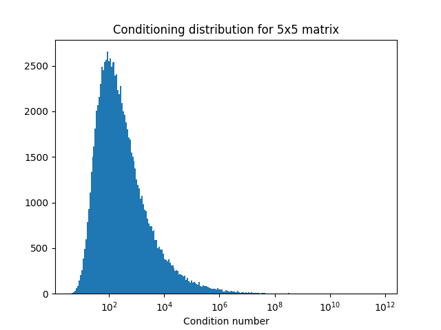
A plot of the condition number across matrices:

Avoiding the issue

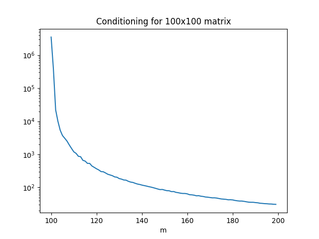
If this is indeed the issue for your solver, you could generate matrices with better eigenvalue distributions. A very simple way to improve the conditioning (flatten the eigenvalue distribution) is to make your initial matrix $H$ non-square ($n \times m$ with $m > n$).

I plotted the condition number for varying $m$, averaged over 100 matrices. We see that it improves the condition number very quickly (note the log scale!).

Please tell me if it helps with your solver.

Answer 3

MOSEK offers a whitepaper on quadratic constraints in which it is concluded that if $Q$ has a suitable factor model, then it is often beneficial to represent your model in a way that exploits this factor model. In your case you have $Q=H^T H$ and although $H$ has no particular properties of interest (besides full rank with high probability), I suggest you try to reformulate $$ \frac{1}{2} x^T Q x + q^T x + q_0 \leq 0 $$

as $$ \frac{1}{2} y^T y + q^T x + q_0 \leq 0,\quad y = Hx, $$

or perhaps even better as $$ \frac{1}{2} y^T y + p^T y + q_0 \leq 0,\quad y = Hx, $$

where $p$ is the solution to $H^T p = q$, such that $p^T y = p^T H x = q^T x$ by definition. In your case, the potential benefit comes from having the quadratic coefficient matrix (the only nonlinear part) becoming an identity matrix which is numerically stable. There is no eigenvalue distribution to worry about.