This question has been asked on Cross Validated

Introduction

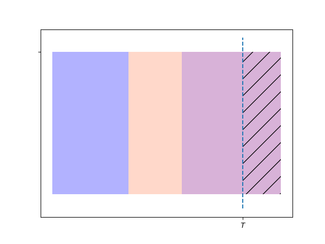
Service is allocated to an infinite source of customers i.e. there is always a service in progress. The duration of the $i^{th}$ service is generally distributed $\Delta_i \sim F_{\Delta}$ where $F_{\Delta}:\mathbb{R}_{\geq0} \to \mathbb{R}[0,1]$ is a uni-variate cumulative distribution function (cdf). This successive service process is illustrated below. An event occurrence (old customer out, new customer in) evolves as follows. $$ t_{k+1} = t_k + \Delta_k $$

The process operates long enough to be in a steady-state or to have reached a stationary distribution. The process is then interrupted at time $T$ for inspection. Upon inspection, the interrupted service has an age $\tau_k = T-t_{k}$ and remaining lifetime $r_k = t_{k+1}-T = t_k + \Delta_k - T$.

I am interested in obtaining distributions for both $\tau_k$ and $r_k$. I have done so algebraically and via simulation. I will provide both the simulation in Python as well as the expressions.

I believe my expressions are correct but something if wrong with my simulations as some bias is introduced. It bothers me as the simulation is very simple but I'm obviously missing something. Please follow along and help me identify the source of error.

Algebraic expressions

Let $F_u$ be a uniform cdf defined over the interval $[0,F_{\Delta}^{-1}(\alpha)]$ where $\alpha$ is almost 1 but slightly less. This is done because $F_{\Delta}$ may have a domain unbounded to the right. Let $f_u$ be its probability density function (pdf) while $f_{\Delta}$ is the service pdf of $F_{\Delta}$. We have a pdf for age of the interrupted process $$ f_{\tau}(\tau) = \frac{1}{\eta}f_{u}(\tau)\left( 1-F_{\Delta}(\tau) \right) $$ where $\eta$ is a normalising constant. For the remaining age $r$ we use convolution because $r = \Delta - \tau$ $$ \begin{align} f_{r}(r) & = \frac{1}{\eta}\left(f_{\Delta}*f_{\tau} \right)(r)\\ & = \frac{1}{\eta}\int_{0}^\infty f_{\Delta}(r+\tau)\, f_{\tau}(\tau)\,d\tau \end{align} $$

Simulation

In the simulation, I allowed $t_k$ to evolve until $t_{k+1} \geq T$. I then terminated and recorded $\tau = T - t_k$ and $t_{k+1} - T$. This is then repeated several times in order to plot normalised histograms as simulated pdfs.

import numpy as np
import matplotlib.pyplot as plt
from scipy.stats import norm,uniform,gamma
from scipy.integrate import quad


def get_interrupted_service(service,T):
    '''Helper function: single run simulation'''
    t = 0
    while True:
        delta = service.rvs()
        # if t + delta > T:
        if t + delta >= T:
            break
        t += delta
    age = T - t
    remain = delta - age
    # remain = t + delta - T
    return age,remain,delta



def sample_interrupted_services(service,T,n_samples):
    '''Main function: collects statistics from independent runs'''
    ages = np.zeros(n_samples)
    remains = np.zeros(n_samples)
    deltas = np.zeros(n_samples)
    for i in range(n_samples):
        if i %10 == 0:
            print('{0} of {1}'.format(i+1,n_samples))
        ages[i],remains[i],deltas[i] = get_interrupted_service(service,T)
    return ages,remains,deltas

I also add the numerical computations of the algebraic expressions.

def get_age_density(service,alpha=0.99):
    uni = uniform(loc=0,scale=service.ppf(alpha))
    def f(t,norm):  
        return uni.pdf(t)*service.sf(t)/norm
    norm = quad(func=lambda t: f(t,1),
                a=0,b=service.ppf(alpha))[0]
    return lambda t: f(t,norm)



def get_remainder_density(service,alpha=0.99):
    age_pdf = get_age_density(service,alpha)
    def convolution(r,norm):
        return (quad(lambda age: service.pdf(r+age)*age_pdf(age),
                     a=0,b=np.inf)[0])/norm
    norm = quad(lambda r:convolution(r,1),
                a=0,b=np.inf)[0]
    return lambda r: convolution(r,norm)

Results

The code is run as follows.

if __name__ == '__main__':
    # Setup simulation
    alpha = 0.9999  # almost 1 e.g. 1 - 1e-6
    f_delta = gamma(a=7,scale=2)
    T = 10000   # Run long enough to reach steady state (bit extreme maybe?)
    samples = 5000  # Need a reasonable amount of iid samples
    # Perform simulation
    tau,r,delta = sample_interrupted_services(f_delta,T,samples)
    # Plot empirical pdfs
    fig,ax = plt.subplots(3,1)
    ax[0].hist(tau,bins=80,density=True,alpha=0.5,label='simulated ages')
    ax[1].hist(r,bins=80,density=True,alpha=0.5,label='simulated remainder')
    ax[2].hist(delta,bins=80,density=True,alpha=0.5,label='simulated service durations')
    # Plot algebraic counterparts for comparison
    t = np.linspace(0,f_delta.ppf(alpha),100)
    age_pdf = get_age_density(f_delta,alpha)
    ax[0].plot(t,age_pdf(t),label='ages')
    r_pdf = get_remainder_density(f_delta,alpha)
    ax[1].plot(t,[r_pdf(ti) for ti in t],label='remainder')  # SLOW !!!
    ax[2].plot(t,f_delta.pdf(t),label='service durations')
    # Show legend/labels
    _ = [ax[i].legend(loc='upper right') for i in range(3)]
    fig.show()
    # Assess bias
    actual_mean = f_delta.mean()
    empirical_mean = delta.mean()
    bias = empirical_mean - actual_mean
    print('actual mean: 'actual_mean)
    print('empirical mean: ',empirical_mean)
    print('bias: ',bias) # should be close to zero.

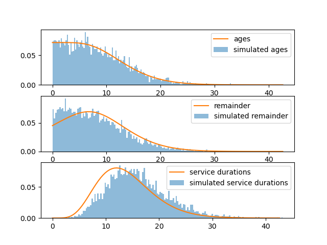
This produces the following. The concern now becomes clear once one looks at the bottom plot. Why is the simulated service duration pdf so biased to the right?. If I look at the middle plot, the misfit is probably due to this bias. I must have not done the simulation properly. Please help me identify the errors.