deleted 110 characters in body
Source Link
Hexaly
  • 3.1k
  • 1
  • 12
  • 17

If you want to implement an algorithm byon your own, then we suggest you a randomized, derivative-free search, even simpler than a Nelder-Mead approachesapproach. Given a feasible solution (respecting the sum equal to 1), move randomly the values of the variables by an epsilon while maintaining the constraint feasible. If the solution is better, then keep it,it; otherwise, throw it away. Start with this simple approach. To go further:, tune the wayhow you choose the epsilons to move, accept less good solutions along the search to diversify (as done in simulated annealing), restartingand restart the search.

LocalSolverHexaly (ex LocalSolver), our global optimization solver, combines several optimization techniques under the hood. Here, the above is essentially what allows LocalSolverHexaly to perform very well on your problem. Thanks to the small number of dimensions (only 3 variables), there is no need to use derivatives (even approximated) to guide and speed up the search. In the same way, there is no need offor surrogate modeling of the cost function because this one is extremely fast to evaluate (about 10,000 calls per second).

Disclaimer: LocalSolverHexaly is a commercial software. You can try it for free duringfor 1 month. In addition, LocalSolverHexaly is free for basic research and teaching.

Please find below the results obtained by LocalSolver,Hexaly using your cost function as external functionexternal function:

function model() {
    X[0..2] <- float(0,1);
    constraint sum[i in 0..2](X[i]) == 1;
    func <- doubleExternalFunction(cost);
    obj <- call(func, X);
    minimize obj;
}

Having declared the cost function, LocalSolverHexaly solves the problem as is. Here "solve" means that LocalSolverHexaly will try to find the best feasible solution to the problem. You can also specify lower and upper bounds for the cost function so that LocalSolverHexaly computes an optimality gap, and then possibly proves the optimality of the solution found.

You can write your model using the LocalSolver modeling languageHexaly modeling language (namely LSP) or using Python, Java, C#, or C++ APIsPython, Java, C#, or C++ APIs. Here is the link to download the LSP file: https://www.localsolver.com/misc/emma.lsphttps://www.hexaly.com/misc/emma.lsp. Having installed LocalSolverHexaly, you can run it using the command "localsolver"hexaly emma.lsp" in console. The best solution found by LocalSolverHexaly after a few seconds on a basic laptop is:

cost = -4683181.09020784, X0 = 0.00106356929433748, X1 = 0.287235884100486, X2 = 0.711702039130129

The sum over the X is equal toequals 1.00000149252495, which is slightly above 1, because LocalSolverHexaly uses a tolerance to satisfy constraints. If you wish the sum over the X to be surely lower than 1, then you can set "< 1" in the above model instead of "== 1". In this case, you will find the following solution:

cost = -4683175.50600612, X0 = 0.00111513425966878, X1 = 0.286966585180356, X2 = 0.711915927974678

Now, the sum over the X is equal to 0.999997647414703.
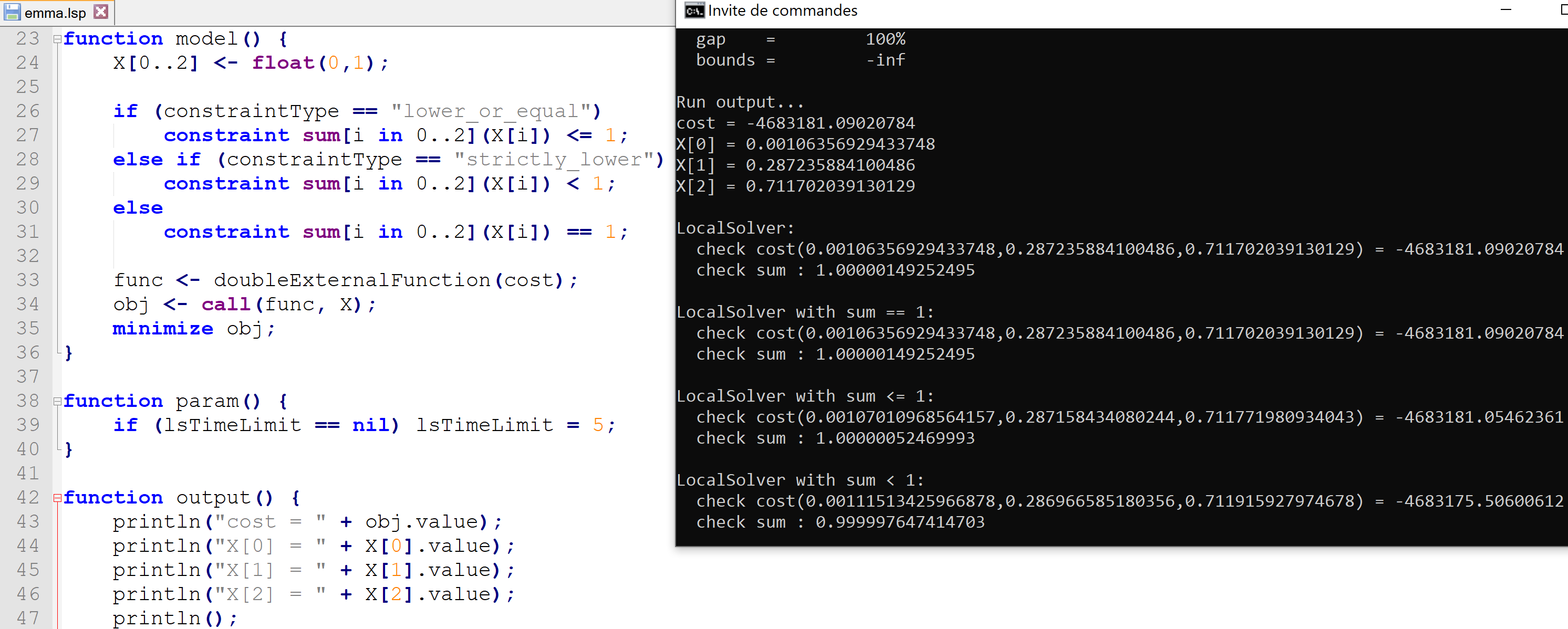
enter image description here

If you want to implement an algorithm by your own, then we suggest you a randomized, derivative-free search, even simpler than Nelder-Mead approaches. Given a feasible solution (respecting the sum equal to 1), move randomly the values of the variables by an epsilon while maintaining the constraint feasible. If the solution is better, then keep it, otherwise throw it. Start with this simple approach. To go further: tune the way you choose the epsilons to move, accept less good solutions along the search to diversify (as done in simulated annealing), restarting the search.

LocalSolver, our global optimization solver, combines several optimization techniques under the hood. Here the above is essentially what allows LocalSolver to perform very well on your problem. Thanks to the small number of dimensions (only 3 variables), there is no need to use derivatives (even approximated) to guide and speed up the search. In the same way, there is no need of surrogate modeling of the cost function because this one is extremely fast to evaluate (about 10,000 calls per second).

Disclaimer: LocalSolver is a commercial software. You can try it for free during 1 month. In addition, LocalSolver is free for basic research and teaching.

Please find below the results obtained by LocalSolver, using your cost function as external function:

function model() {
    X[0..2] <- float(0,1);
    constraint sum[i in 0..2](X[i]) == 1;
    func <- doubleExternalFunction(cost);
    obj <- call(func, X);
    minimize obj;
}

Having declared the cost function, LocalSolver solves the problem as is. Here "solve" means that LocalSolver will try to find the best feasible solution to the problem. You can also specify lower and upper bounds for the cost function so that LocalSolver computes an optimality gap, and then possibly proves the optimality of the solution found.

You can write your model using the LocalSolver modeling language (namely LSP) or using Python, Java, C#, or C++ APIs. Here is the link to download the LSP file: https://www.localsolver.com/misc/emma.lsp. Having installed LocalSolver, you can run it using the command "localsolver emma.lsp" in console. The best solution found by LocalSolver after a few seconds on a basic laptop is:

cost = -4683181.09020784, X0 = 0.00106356929433748, X1 = 0.287235884100486, X2 = 0.711702039130129

The sum over the X is equal to 1.00000149252495, which is slightly above 1, because LocalSolver uses a tolerance to satisfy constraints. If you wish the sum over the X to be surely lower than 1, then you can set "< 1" in the above model instead of "== 1". In this case, you will find the following solution:

cost = -4683175.50600612, X0 = 0.00111513425966878, X1 = 0.286966585180356, X2 = 0.711915927974678

Now the sum over the X is equal to 0.999997647414703.

enter image description here

If you want to implement an algorithm on your own, then we suggest a randomized, derivative-free search, even simpler than a Nelder-Mead approach. Given a feasible solution (respecting the sum equal to 1), move randomly the values of the variables by an epsilon while maintaining the constraint feasible. If the solution is better, keep it; otherwise, throw it away. Start with this simple approach. To go further, tune how you choose the epsilons to move, accept less good solutions along the search to diversify (as done in simulated annealing), and restart the search.

Hexaly (ex LocalSolver), our global optimization solver, combines several optimization techniques under the hood. Here, the above essentially allows Hexaly to perform very well on your problem. Thanks to the small number of dimensions (only 3 variables), there is no need to use derivatives (even approximated) to guide and speed up the search. In the same way, there is no need for surrogate modeling of the cost function because this one is extremely fast to evaluate (about 10,000 calls per second).

Disclaimer: Hexaly is commercial software. You can try it for free for 1 month. In addition, Hexaly is free for basic research and teaching.

Please find below the results obtained by Hexaly using your cost function as external function:

function model() {
    X[0..2] <- float(0,1);
    constraint sum[i in 0..2](X[i]) == 1;
    func <- doubleExternalFunction(cost);
    obj <- call(func, X);
    minimize obj;
}

Having declared the cost function, Hexaly solves the problem as is. Here "solve" means that Hexaly will try to find the best feasible solution to the problem. You can also specify lower and upper bounds for the cost function so that Hexaly computes an optimality gap and then possibly proves the optimality of the solution found.

You can write your model using the Hexaly modeling language (namely LSP) or using Python, Java, C#, or C++ APIs. Here is the link to download the LSP file: https://www.hexaly.com/misc/emma.lsp. Having installed Hexaly, you can run it using the command "hexaly emma.lsp" in console. The best solution found by Hexaly after a few seconds on a basic laptop is:

cost = -4683181.09020784, X0 = 0.00106356929433748, X1 = 0.287235884100486, X2 = 0.711702039130129

The sum over the X equals 1.00000149252495, slightly above 1, because Hexaly uses a tolerance to satisfy constraints. If you wish the sum over the X to be surely lower than 1, then you can set "< 1" in the above model instead of "== 1". In this case, you will find the following solution:

cost = -4683175.50600612, X0 = 0.00111513425966878, X1 = 0.286966585180356, X2 = 0.711915927974678

Now, the sum over the X is equal to 0.999997647414703.

enter image description here

added 4 characters in body
Source Link
SecretAgentMan
  • 1.9k
  • 2
  • 14
  • 39

If you want to implement an algorithm by your own, then we suggest you a randomized, derivative-free search, even simpler than Nelder-Mead approaches. Given a feasible solution (respecting the sum equal to 1), move randomly the values of the variables by an epsilon while maintaining the constraint feasible. If the solution is better, then keep it, otherwise throw it. Start with this simple approach. To go further: tune the way you choose the epsilons to move, accept less good solutions along the search to diversify (as done in simulated annealing), restarting the search.

LocalSolver, our global optimization solver, combines several optimization techniques under the hood. Here the above is essentially what allows LocalSolver to perform very well on your problem. Thanks to the small number of dimensions (only 3 variables), there is no need to use derivatives (even approximated) to guide and speed up the search. In the same way, there is no need of surrogate modeling of the cost function because this one is extremely fast to evaluate (about 10,000 calls per second).

Disclaimer:Disclaimer: LocalSolver is a commercial software. You can try it for free during 1 month. In addition, LocalSolver is free for basic research and teaching.

Please find below the results obtained by LocalSolver, using your cost function as external function:

function model() {
    X[0..2] <- float(0,1);
    constraint sum[i in 0..2](X[i]) == 1;
    func <- doubleExternalFunction(cost);
    obj <- call(func, X);
    minimize obj;
}

Having declared the cost function, LocalSolver solves the problem as is. Here "solve" means that LocalSolver will try to find the best feasible solution to the problem. You can also specify lower and upper bounds for the cost function so that LocalSolver computes an optimality gap, and then possibly proves the optimality of the solution found.

You can write your model using the LocalSolver modeling language (namely LSP) or using Python, Java, C#, or C++ APIs. Here is the link to download the LSP file: https://www.localsolver.com/misc/emma.lsp. Having installed LocalSolver, you can run it using the command "localsolver emma.lsp" in console. The best solution found by LocalSolver after a few seconds on a basic laptop is:

cost = -4683181.09020784, X0 = 0.00106356929433748, X1 = 0.287235884100486, X2 = 0.711702039130129

The sum over the X is equal to 1.00000149252495, which is slightly above 1, because LocalSolver uses a tolerance to satisfy constraints. If you wish the sum over the X to be surely lower than 1, then you can set "< 1" in the above model instead of "== 1". In this case, you will find the following solution:

cost = -4683175.50600612, X0 = 0.00111513425966878, X1 = 0.286966585180356, X2 = 0.711915927974678

Now the sum over the X is equal to 0.999997647414703.

enter image description here

If you want to implement an algorithm by your own, then we suggest you a randomized, derivative-free search, even simpler than Nelder-Mead approaches. Given a feasible solution (respecting the sum equal to 1), move randomly the values of the variables by an epsilon while maintaining the constraint feasible. If the solution is better, then keep it, otherwise throw it. Start with this simple approach. To go further: tune the way you choose the epsilons to move, accept less good solutions along the search to diversify (as done in simulated annealing), restarting the search.

LocalSolver, our global optimization solver, combines several optimization techniques under the hood. Here the above is essentially what allows LocalSolver to perform very well on your problem. Thanks to the small number of dimensions (only 3 variables), there is no need to use derivatives (even approximated) to guide and speed up the search. In the same way, there is no need of surrogate modeling of the cost function because this one is extremely fast to evaluate (about 10,000 calls per second).

Disclaimer: LocalSolver is a commercial software. You can try it for free during 1 month. In addition, LocalSolver is free for basic research and teaching.

Please find below the results obtained by LocalSolver, using your cost function as external function:

function model() {
    X[0..2] <- float(0,1);
    constraint sum[i in 0..2](X[i]) == 1;
    func <- doubleExternalFunction(cost);
    obj <- call(func, X);
    minimize obj;
}

Having declared the cost function, LocalSolver solves the problem as is. Here "solve" means that LocalSolver will try to find the best feasible solution to the problem. You can also specify lower and upper bounds for the cost function so that LocalSolver computes an optimality gap, and then possibly proves the optimality of the solution found.

You can write your model using the LocalSolver modeling language (namely LSP) or using Python, Java, C#, or C++ APIs. Here is the link to download the LSP file: https://www.localsolver.com/misc/emma.lsp. Having installed LocalSolver, you can run it using the command "localsolver emma.lsp" in console. The best solution found by LocalSolver after a few seconds on a basic laptop is:

cost = -4683181.09020784, X0 = 0.00106356929433748, X1 = 0.287235884100486, X2 = 0.711702039130129

The sum over the X is equal to 1.00000149252495, which is slightly above 1, because LocalSolver uses a tolerance to satisfy constraints. If you wish the sum over the X to be surely lower than 1, then you can set "< 1" in the above model instead of "== 1". In this case, you will find the following solution:

cost = -4683175.50600612, X0 = 0.00111513425966878, X1 = 0.286966585180356, X2 = 0.711915927974678

Now the sum over the X is equal to 0.999997647414703.

enter image description here

deleted 13 characters in body
Source Link
Hexaly
  • 3.1k
  • 1
  • 12
  • 17
function model() {
    N = 3;
    X[0..N-1]2] <- float(0,1);
    constraint sum[i in 0..N-1]2](X[i]) == 1;
    func <- doubleExternalFunction(cost);
    obj <- call(func, X);
    minimize obj;
}

You can write your model using the LocalSolver modeling language (namely LSP) or using Python, Java, C#, or C++ APIs. Here is the link to download the LSP file: https://www.localsolver.com/misc/emma.lsp. Having installed LocalSolver, you can run it using the command "localsolver emma.lsp" in console. The best solution found by LocalSolver after a few seconds on a basic laptop is:

cost = -46831554683181.09020784, X0 = 0.001215763250076500106356929433748, X1 = 0.286070665348843287235884100486, X2 = 0.712713571407526711702039130129

ThisThe sum over the X is better thanequal to 1.00000149252495, which is slightly above 1, because LocalSolver uses a tolerance to satisfy constraints. If you wish the ones found by you usingsum over the SciPy SLSQP method andX to be surely lower than 1, then by prubin usingyou can set "< 1" in the above model instead of "== 1". In this case, you will find the following solution:

cost = Nelder-Mead downhill simplex method-4683175.50600612, whileX0 = 0.00111513425966878, X1 = 0.286966585180356, X2 = 0.711915927974678

Now the sum over the X variables is much closerequal to 1:0.999997647414703.

  • cost = -4495453, X0 = 0.17023975, X1 = 0.19532928, X2 = 0.64296507
  • cost = -4675913, X0 = 0.0126960, X1 = 0.2461336, X2 = 0.7411704

enter image description hereenter image description here

function model() {
    N = 3;
    X[0..N-1] <- float(0,1);
    constraint sum[i in 0..N-1](X[i]) == 1;
    func <- doubleExternalFunction(cost);
    obj <- call(func, X);
    minimize obj;
}

You can write your model using the LocalSolver modeling language (namely LSP) or using Python, Java, C#, or C++ APIs. Here is the link to download the LSP file: https://www.localsolver.com/misc/emma.lsp. The best solution found by LocalSolver is:

cost = -4683155, X0 = 0.0012157632500765, X1 = 0.286070665348843, X2 = 0.712713571407526

This is better than the ones found by you using the SciPy SLSQP method and then by prubin using the Nelder-Mead downhill simplex method, while the sum over the X variables is much closer to 1:

  • cost = -4495453, X0 = 0.17023975, X1 = 0.19532928, X2 = 0.64296507
  • cost = -4675913, X0 = 0.0126960, X1 = 0.2461336, X2 = 0.7411704

enter image description here

function model() {
    X[0..2] <- float(0,1);
    constraint sum[i in 0..2](X[i]) == 1;
    func <- doubleExternalFunction(cost);
    obj <- call(func, X);
    minimize obj;
}

You can write your model using the LocalSolver modeling language (namely LSP) or using Python, Java, C#, or C++ APIs. Here is the link to download the LSP file: https://www.localsolver.com/misc/emma.lsp. Having installed LocalSolver, you can run it using the command "localsolver emma.lsp" in console. The best solution found by LocalSolver after a few seconds on a basic laptop is:

cost = -4683181.09020784, X0 = 0.00106356929433748, X1 = 0.287235884100486, X2 = 0.711702039130129

The sum over the X is equal to 1.00000149252495, which is slightly above 1, because LocalSolver uses a tolerance to satisfy constraints. If you wish the sum over the X to be surely lower than 1, then you can set "< 1" in the above model instead of "== 1". In this case, you will find the following solution:

cost = -4683175.50600612, X0 = 0.00111513425966878, X1 = 0.286966585180356, X2 = 0.711915927974678

Now the sum over the X is equal to 0.999997647414703.

enter image description here

deleted 73 characters in body
Source Link
Hexaly
  • 3.1k
  • 1
  • 12
  • 17
Loading
deleted 73 characters in body
Source Link
Hexaly
  • 3.1k
  • 1
  • 12
  • 17
Loading
deleted 1 character in body
Source Link
Hexaly
  • 3.1k
  • 1
  • 12
  • 17
Loading
added 1055 characters in body
Source Link
Hexaly
  • 3.1k
  • 1
  • 12
  • 17
Loading
The answer has been completed: a code snippet is given and the solution found by LocalSolver
Source Link
Hexaly
  • 3.1k
  • 1
  • 12
  • 17
Loading
Source Link
Hexaly
  • 3.1k
  • 1
  • 12
  • 17
Loading