8
$\begingroup$

I have a linear optimization problem for which I am looking for a suitable optimization solution that can fulfill my requirements. Here is an explanation of the optimization problem:

There are a number of n variables x1, x2, .., xn relevant for the optimization. They contain a value between 0 and 100, whereby the sum of the variables is always 100%. The variables are used as multiplication coefficient for their respective vector with m entries.

There are different functions for determining the cost value for the variables depending on the optimization goal. One of them is shown below as a pseudo code:

cost_function(x1, x2, .., xn)
       i = 0
       min_value = 0
       **while** i < m
           e = x0 * E0_i + x1 * E1_i + .. + xn * EN_i
           v = (s0 * E0_i + s1 * E1_i + .. + sn * EN_i) / e
           minimize_value += min(-C_i, e) * (P_i - v)
       **return** minimize_value

where the bold characters represent vectors and the other scalar values.

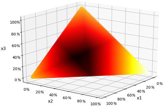
The diagram shows the state space with three variables x1, x2 and x3, where darker is better:

enter image description here

Currently, I use Simulated Annealing for this optimization problem, but the state s' is only accepted as new state if it is better than s, because it would be counterproductive to have a probability to take over worse states in a linear optimization problem. From a scientific point of view, the use of Simulated Annealing is probably not appropriate for the application.

Would linear programming still be recommended in this case? Or is there an alternative to Simulated Annealing for linear optimization problems?


EDIT:

A minimum working example of the problem can be found here

The result of the variables should be: [0.17023975 0.19532928 0.64296507]

$\endgroup$
9
  • $\begingroup$ Are s0...sn and C constants? Is v in line 9 computed using the i-th component of each E vector (as written, v would be a vector, unless the si were vectors and * meant inner product)? Are the P_i constants? $\endgroup$
    – prubin
    Commented May 23, 2020 at 17:26
  • $\begingroup$ @Emma, what exactly do you mean by linear programming? What you mentioned is a metaheuristic and is quite different from exact methods like LP. If you are interested to use LP/MIP, you should try writing your problem in those formats and ask your question again if you would have any issues. :) $\endgroup$
    – A.Omidi
    Commented May 24, 2020 at 9:11
  • $\begingroup$ @prubin Yes, s0..sn are constant scalars and C is a constant vector. The operator * in line 9 means the multiplication of a scalar by a vector. P_i are constants. Sorry for the confusion. $\endgroup$
    – Emma
    Commented May 24, 2020 at 9:36
  • 1
    $\begingroup$ Do you have a minimum working example of the problem implemented in a way you could upload? $\endgroup$
    – Richard
    Commented May 27, 2020 at 20:05
  • 1
    $\begingroup$ @Emma: The minimum is actually quite helpful, because it allows you to rewrite min(C_i, e) * (P_i - v) as e * (P_i - v) with the constraint that e<=C_i. This gets you close to having a quadratic program, which you can solve efficiently and exactly. However, looking at the values of C[i] in your example and the constraint that x>=0, it will always be the case that min(C_i,e)=C_i. Are you sure this objective function is correct? $\endgroup$
    – Richard
    Commented May 29, 2020 at 6:34

2 Answers 2

14
+50
$\begingroup$

First, the problem is not a linear optimization problem, at least not for the objective function shown (which is nonlinear due the conditional portion in lines 10-13 and particularly the division by E_ges_i in line 13. Simulated annealing might be fine as a heuristic approach, but given the nonlinear objective, only accepting improving steps might or might not be appropriate. If the objective is unimodal, I think skipping steps that make the objective worse might be okay. Then again, if the heat map is unimodal, constrained gradient descent might work just as well or better.

Sticking to the objective function shown, another possibility would be to treat the problem as a mixed integer linear program, using a piecewise linear approximation to the objective function. Since an approximation is involved, you might want to try gradient descent or other local search from the model's solution to see if you can improve it, or alternatively refine the approximation near the model solution and solve the revised model (ad nauseum).

ADDENDUM: I just hacked a little R code, using the objective function posted on GitHub. The algorithm I used is the Nelder-Mead polytope algorithm, as described in 1. The Nelder-Mead algorithm, published in 1965, was a modification of an earlier algorithm (by Spendley, Hext and Himsworth in 1962, according to 1) and has likely been improved upon in turn since the '60s. The attraction of the Nelder-Mead algorithm (or its relatives) here is that it starts with a simplex as the search region and progressively shrinks to smaller and smaller simplices, all of which are subsets of the original. So if we use N-M starting with the unit simplex, the constraints are always satisfied.

I did not put in much care in the coding, did not code all the possible adjustments (such as random restarts), and picked the expansion, contraction and reflection parameters out of thin air. That said, it converged (or at least stopped) after seven iterations on the test problem, with a solution of (0.0126960, 0.2461336, 0.7411704) and an objective value of -4675913 -- not optimal, but I think not too shabby (particularly since I did not code restarts or other more recent tweaks to Nelder-Mead). It's not hard to code, and it does not require derivatives, just function evaluations.

1 P. Gill, W. Murray and M. Wright, Practical Optimization (Academic Press, 1981).

ADDENDUM 2 I updated my R code to use the simplified version of the cost function from the GitHub repository (which is a bit better behaved when an argument is zero). I also switched from the Nelder-Mead algorithm as present in Gill, Murray and Wright to the version on the Wikipedia page, and adjusted the parameter values to the ones they recommend. I have to qualify my earlier comment about Nelder-Mead automatically maintaining feasibility. The condition that the weights sum to 1 is automatically maintained. Nonnegativity of the weights requires occasionally shrink a proposed step, which is easily handled.

With the modified code and the parameter values from the Wikipedia page, I get a final solution of (0, 0.2885719, 0.7114281) with an objective value of -4,683,095.

ADDENDUM 3 Hopefully this will be my final addendum. :-) I also tried a genetic algorithm (in R). The solution from a GA is inherently random, but with the parameters and random seed that I chose I got a final solution of (0.001182725, 0.2869361, 0.7118812) with objective value -4,683,175, which is slightly better than both what I got with Nelder-Mead and what LocalSolver reported.

My R code for both Nelder-Mead and the GA (using the genalg R library) are available in an R notebook.
$\endgroup$
16
  • 1
    $\begingroup$ It should be alright, SLSQP works quite well for local optimization of nonlinear constrained problems. Nonetheless, I'd also consider @prubin's proposal of using constrained gradient descent, as it should be faster than solving a sequence of QP's. I might be biased: tend to prefer - from all approaches that work - the one that's simpler or less restrictive. Emma, here and here you can find info about SLSQP (how it works, requirements and check when it can be used). $\endgroup$
    – dhasson
    Commented May 27, 2020 at 1:05
  • 1
    $\begingroup$ @Emma you're welcome. Do you refer to gradient descent pseudocode (as the function in your question) or implementation in a particular language? $\endgroup$
    – dhasson
    Commented May 27, 2020 at 18:41
  • 1
    $\begingroup$ @LocalSolver The comment above doesn't belong on prubin's answer. It can be a comment on the question (rather than on an answer), but since you are essentially answering the question, it's really better if you post it as a new answer, not a comment. Please delete your comment and repost as a comment on the question, or as a separate answer. $\endgroup$ Commented May 29, 2020 at 2:27
  • 1
    $\begingroup$ FYI. Gill, Murray, Wright "Practical Optimization" has recently been reprinted by SIAM my.siam.org/Store/Product/viewproduct/?ProductId=31205265 . $\endgroup$ Commented May 29, 2020 at 12:25
  • 1
    $\begingroup$ @Emma I just updated my answer with results from a GA (even better) and a link to my R code. If you have questions about it, the home page for site where the R code exists has my contact info on it. $\endgroup$
    – prubin
    Commented May 31, 2020 at 20:42
6
$\begingroup$

If you want to implement an algorithm on your own, then we suggest a randomized, derivative-free search, even simpler than a Nelder-Mead approach. Given a feasible solution (respecting the sum equal to 1), move randomly the values of the variables by an epsilon while maintaining the constraint feasible. If the solution is better, keep it; otherwise, throw it away. Start with this simple approach. To go further, tune how you choose the epsilons to move, accept less good solutions along the search to diversify (as done in simulated annealing), and restart the search.

Hexaly (ex LocalSolver), our global optimization solver, combines several optimization techniques under the hood. Here, the above essentially allows Hexaly to perform very well on your problem. Thanks to the small number of dimensions (only 3 variables), there is no need to use derivatives (even approximated) to guide and speed up the search. In the same way, there is no need for surrogate modeling of the cost function because this one is extremely fast to evaluate (about 10,000 calls per second).

Disclaimer: Hexaly is commercial software. You can try it for free for 1 month. In addition, Hexaly is free for basic research and teaching.

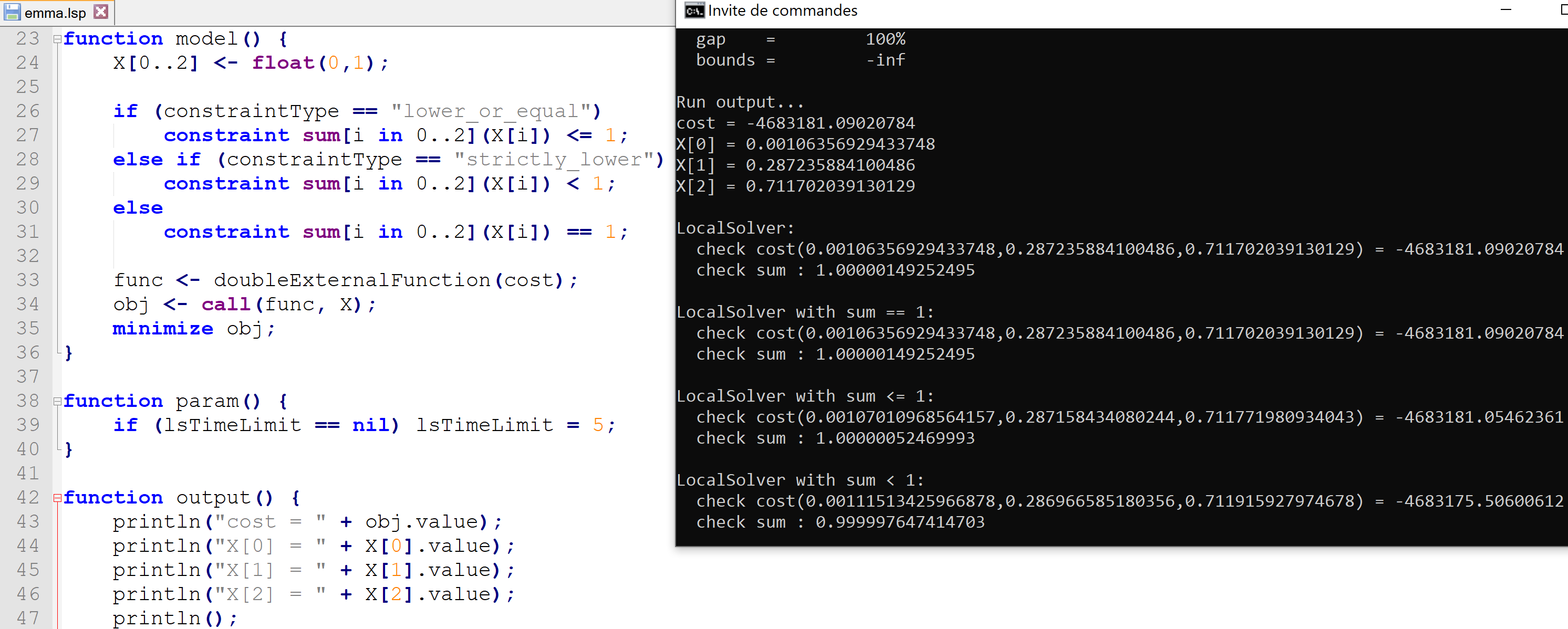
Please find below the results obtained by Hexaly using your cost function as external function:

function model() {
    X[0..2] <- float(0,1);
    constraint sum[i in 0..2](X[i]) == 1;
    func <- doubleExternalFunction(cost);
    obj <- call(func, X);
    minimize obj;
}

Having declared the cost function, Hexaly solves the problem as is. Here "solve" means that Hexaly will try to find the best feasible solution to the problem. You can also specify lower and upper bounds for the cost function so that Hexaly computes an optimality gap and then possibly proves the optimality of the solution found.

You can write your model using the Hexaly modeling language (namely LSP) or using Python, Java, C#, or C++ APIs. Here is the link to download the LSP file: https://www.hexaly.com/misc/emma.lsp. Having installed Hexaly, you can run it using the command "hexaly emma.lsp" in console. The best solution found by Hexaly after a few seconds on a basic laptop is:

cost = -4683181.09020784, X0 = 0.00106356929433748, X1 = 0.287235884100486, X2 = 0.711702039130129

The sum over the X equals 1.00000149252495, slightly above 1, because Hexaly uses a tolerance to satisfy constraints. If you wish the sum over the X to be surely lower than 1, then you can set "< 1" in the above model instead of "== 1". In this case, you will find the following solution:

cost = -4683175.50600612, X0 = 0.00111513425966878, X1 = 0.286966585180356, X2 = 0.711915927974678

Now, the sum over the X is equal to 0.999997647414703.

enter image description here

$\endgroup$
5
  • 5
    $\begingroup$ I think it would be constructive if downvoters explained why they down voted : is this solution not mathematically relevant ? Or is too much of a "black box" approach, where the black box is a commercial software ? $\endgroup$
    – Kuifje
    Commented May 28, 2020 at 7:23
  • 1
    $\begingroup$ LocalSolver, it's interesting your program found a better solution than @prubin's and Emma's approaches. I wonder how running time and function evaluations compare in the same machine (as it executed 10k+ iterations)? $\endgroup$
    – dhasson
    Commented May 29, 2020 at 2:40
  • 3
    $\begingroup$ @dhasson The results were obtained on a basic laptop. You can reproduce the results on your machine if you are interested in. Here the cost function to is extremely fast to evaluate (about 10,000 evaluations per second). Then a randomized derivative-free search, with all the stuff to diversify and then escape local optima, will perform very well. By experience, it keep on working well with slower functions, with a few evaluations per second. If much slower (a few seconds or more per evaluation), then surrogate modeling of the cost function becomes interesting to avoid calling it too much. $\endgroup$
    – Hexaly
    Commented May 29, 2020 at 9:24
  • 2
    $\begingroup$ @LocalSolver: In my opinion, your paragraph "If you want to implement an algorithm by your own..." is probably what the OP was expecting, as you explain an algorithmic strategy. I would suggest putting this paragraph at the way top. And then, illustrate your point with the example implemented in LocalSolver. I think the answer provided as is is of good quality! $\endgroup$
    – Kuifje
    Commented May 29, 2020 at 10:06
  • $\begingroup$ @Kuifje Thanks a lot for your constructive comment. We correct the post accordingly. Hope that this will be more helpful like this. $\endgroup$
    – Hexaly
    Commented May 29, 2020 at 10:23

Your Answer

By clicking “Post Your Answer”, you agree to our terms of service and acknowledge you have read our privacy policy.

Not the answer you're looking for? Browse other questions tagged or ask your own question.