I'm considering the following basic assignment problem: a group of $n$ people is to be assigned, in one-to-one fashion, a set of $n$ jobs. Write $C_{ij}$ for the cost incurred when person $i$ gets assigned to job $j$. I shall assume that the $C_{ij}$ are iid exponentially distributed.

I consider two greedy algorithms.

• Algorithm A assigns to person 1 the job that results in the least cost, then chooses for person 2 the cheapest job out of the remaining $n-1$ options, and so on.
• Algorithm B considers all $n^2$ cost values, finds the minimal pair $(i_1,j_1)$, and assigns person $i_1$ to job $j_1$, so that $(n-1)^2$ values remain, finds the minimal pair $(i_2,j_2)$ out of those, and so on.

I claim that both algorithms have the same expected cost. By noting that the minimum of $k$ exponentially distributed variables of rate $\mu$ is itself exponentially distributed of rate $k\mu$, one shows that algorithm A has expected cost $$E(A) = 1 + \frac{1}{2} + \cdots + \frac{1}{n}.$$ Now for algorithm B. The minimal cost $C_{(i_1,j_1)}$ is exponentially distributed of rate $n^2$. By memorylessness, $C_{(i_2,j_2)}$ is equal to $C_{(i_1,j_1)}$ plus an exponential of rate $(n-1)^2$, and so on, so that \begin{equation} \begin{split} E(B) &= E(C_{(i_1,j_1)}) + \cdots + E(C_{(i_n,j_n)}) \\ &= n \cdot \frac{1}{n^2} + (n-1)\cdot \frac{1}{(n-1)^2} + \cdots + 1 \cdot \frac{1}{1^2}\\ &= \frac{1}{n} + \frac{1}{n-1} + \cdots + 1. \end{split} \end{equation}

My intuition expecting the global approach to typically be more efficient, I was surprised by this outcome, and attempted to simulate the situation. Let's implement the greedy algorithms in Python.

def GreedyA(arr):
    total_cost = 0
    for _ in range(n - 1):
        job_choices = arr[0]
        cheapest = job_choices.argmin()
        total_cost += job_choices[cheapest]
        arr = np.delete(arr, 0, axis = 0)
        arr = np.delete(arr, cheapest, axis = 1)
    return total_cost

def GreedyB(arr):
    total_cost = 0
    for _ in range(n - 1):
        x, y = np.unravel_index(arr.argmin(), arr.shape)
        total_cost += arr[x][y]
        arr = np.delete(arr, x, axis = 0)
        arr = np.delete(arr, y, axis = 1)
    return total_cost

I now run the simulation, arbitrarily picking $n$ to be $10$, making the math predict that $E(A) = E(B) \approx 2.9$.

values_A = []
values_B = []

n = 10
iterations = 10000

for _ in range(iterations):
    costs = np.random.exponential(size = (n, n), scale = 1)
    outcomeA = GreedyA(costs)
    outcomeB = GreedyB(costs)
    values_A.append(outcomeA)
    values_B.append(outcomeB)

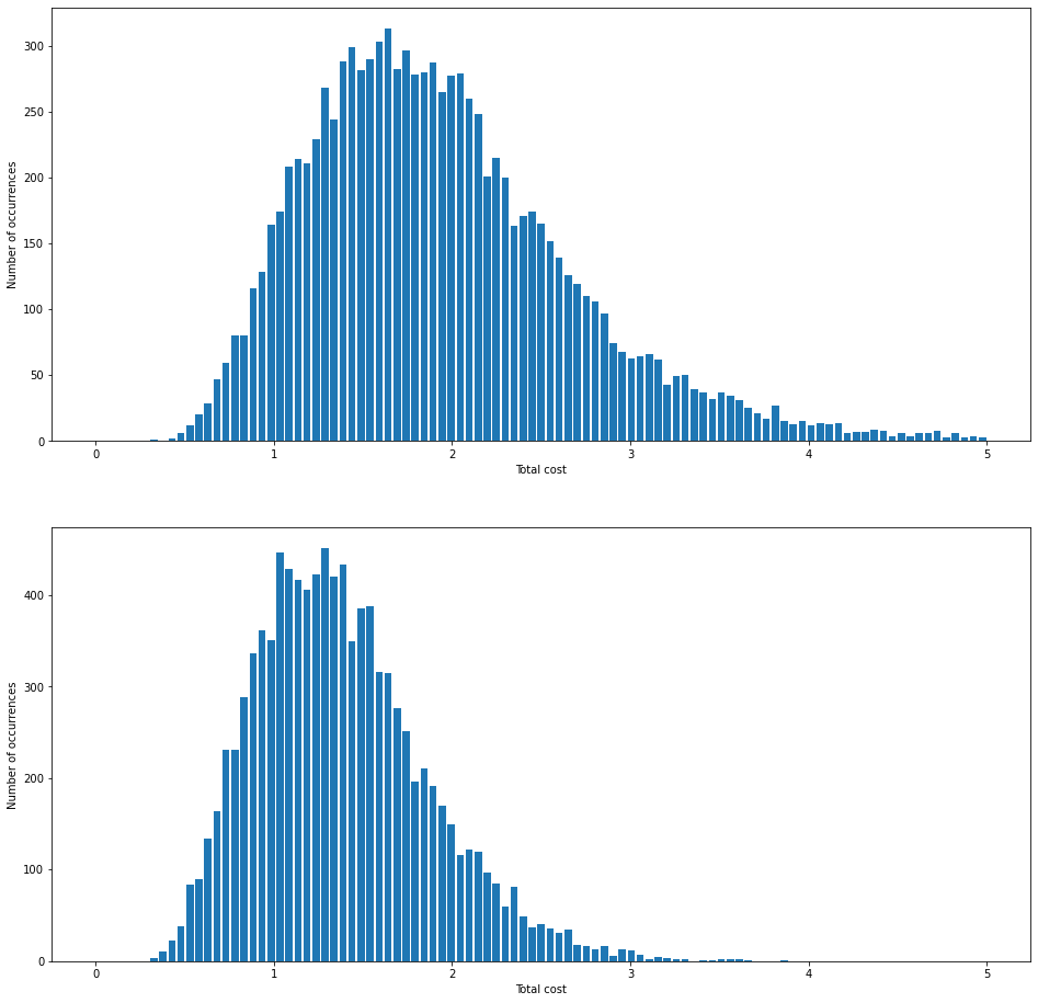
I'll plot the results.

Both algorithms seem to come out more efficiently than expected, as nearly all simulation resulted in a cost significantly below $2.9$. In addition, in line with my doubts, algorithm B seems to perform much better than algorithm A.

Question. What is going wrong in my analysis?